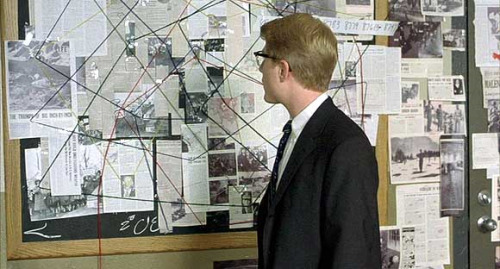
Many readers of the last post requested a more formal definition of a UGF. Let’s look a bit more closely at the definition of an SDF and how it compares to UGFs and other useful fields in engineering applications. Some readers may find the visual concepts more intuitive than the nuances, so let’s get a feel for the territory first by examining the field at the intersection of two planes:
With SDF enabled and offset non-negative, the boundary map arrow always points to the boundary, via the distance intersection of two planes, \(\df{F} = \plane{A} \distanceCap \plane{B}\) . With SDF disabled, the points in a region opposite of the vertex, the normal cone of the intersection, fail to point at the boundary. The normal cone, shown in green, is the set of points closest to the sharp intersection. Similarly, with SDF enabled and negative offset, the boundary map of points in the normal cone of the intersection trace out the classic swallowtail failure mode of offsetting chains of curves with fillets.
 A swallow with its tail
Definitions
Let’s nail down some definitions to at least a SIGGRAPH level of rigor. For nuanced definitions, see Luo, Wang, and Lukens’s framing of SDFs using Variational Analysis.
Fields
Fields are functions mapping a smoothly curved space, usually \(\R^n\), to the affinely extended reals \(\overline\R \equiv \R \cup \{\pm\infty\}\). If you haven’t seen extended reals before, it turns out that you can do the hokey-pokey with analysis and simply define the ends of the real number line to be closed instead of open, even dividing (anything other than zero) by zero; feel free to resent your third grade teachers and find new brilliance in IEEE floating point representations.
Unit Gradient Fields
Unit Gradient Fields (UGFs) are simply fields with unit gradient magnitude, everywhere the gradient exists. Although we usually use them to represent shapes, there is no need for them to have any non-positive values, as adding a constant to a UGF doesn’t change its gradient.
Distance Fields
Distance fields (DFs) are defined by the difference of the unsigned distance to a set minus the unsigned distance to the set’s complement, noting that the distance to a set from its inside is zero. The piecewise definition is \(C^1\) continuous (where differentiable) across the set’s boundary. DFs are UGFs when defined by proper sets. (The two improper sets, the null set and the set of all points in a space, generate the distance fields \(+\infty\) and \(-\infty\), respectively.) When DFs have an interior, we will call them “signed” SDFs. (We avoid the term “UDF” due to its similarity to “UGF”.)
DFs contain more information about a shape than a UGF representing the same shape. For example, the sum of two DFs represents the local clearance between parts. These properties derive from the key fact about DFs: their boundary map always points to their boundary.
The Boundary Map
The boundary map, represented by the black arrow in the visualization, is simply the map from point \(\p\) to the closest point on the surface of a set represented by a DF \(\df{F}\):
\[\BoundaryMap{\df{F}}(\p) = \p - \df{F} \;\, \grad\df{F}\]Distance fields can be thought of as the magnitude of the boundary map vector fields, and any UGF that is a boundary map represents a distance field.
The Normal Cone
We can constuct the normal cone as illustrated above using the boundary map. Given two SDFs \(\df{A}(\p)\) and \(\df{B}(\p)\) the normal cone for \(\ugf{F} = \df{A} \distanceCap \df{B}\) becomes:
\[\NormalCone{\ugf{F}} = -\df{A}\left(\BoundaryMap{\df{B}}(\p)\right) \minmaxCap -\df{B}\left(\BoundaryMap{\df{A}}(\p)\right)\]Plane Fields
Plane fields are a special case of SDFs to planar half-spaces with the special property that they are everywhere differentiable.
Notation
In this series, we’ll use a secondary notation to remind ourselves of the properties of fields:
| Plane fields | \(\plane{P}\) |
| Distance field | \(\df{D}\) |
| Unit gradient field | \(\ugf{U}\) |
| Unit gradient field at zero | \(\augf{A}\) |
Approximate UGFs
The latter, we’ll refer to as approximate UGFs (AUGFs). Any field with non-vanishing gradient can be converted to an AUGF via Sampson normalization (Sampson 1982):
\[\sampson{F} \equiv \frac{F}{\norm{\grad{F}}} \;.\]We will often generalize properties of planar intersections to behavior near the zero isosurface of AUGFs.
Families of Booleans
So far, we’ve seen minmax, distance-based, and, in the last post, chamfered Booleans that preserve UGFness. There are also many useful fast and reliable Boolean operations that produce results that are not UGFs.
We’re going to need some notation to keep the different flavors of Booleans straight. Let’s focus on the Union or \(\min\) operation, as the intersection can be defined as the complement of the union of the complement of the inputs via De Morgan’s law:
\[\max(A, B) = -\min(-A, -B) \;.\]Distance-Preserving Boolean
First, nodding to Rvachev and logic functions, we can define the minmax Booleans \(\minmaxCup\) and \(\minmaxCap\) using \(\min\) and \(\max\). Similarly, we can define the DF-preserving Booleans, \(\distanceCup\) and \(\distanceCap\), which are defined piecewise across the boundary of the normal cone. Outside of the normal cone, the distance result is the same as the minimax Booleans, but inside it sees the distance to the curve of intersection.
Euclidean Blend
It’s worth comparing the DF blend to common implicits blends in the graphics community. Korndörfer gives perhaps the most elegant, in which the entire remote quadrant of the intersection receives the blend instead of the normal cone, a subset of it:
\[\ugf{A} \euclideanCup \ugf{B} \equiv \max\!\left(\ugf{A} \minmaxCup \ugf{B}, 0 \right) \;-\; \norm{\left(\min(\ugf{A}, 0),\strut\min(\ugf{B}, 0) \right)} \;,\]where \(\norm{\cdot}\) is the Euclidean norm of a vector of fields. We’ll use variants of the traditional union and intersections symbols for blended or rounded intersections.
Scaled Quilez Blend
Quilez provide several examples of “smooth minimum functions” that blend the entire discontinuity typically produced by \(\min\). With constant blend radius, they do not repeat the logic of \(\min\) and \(\max\), but by using an estimate of distance-to-curve for their intersection, we can produce a logic-preserving minimum. This radius variation works on Quilez’ polynomial and exponential \(\func{smin}\):
\[\func{smin}\left(\ugf{A}\,, \ugf{B}\,, \abs{\ugf{A} \, \ugf{B } \; (1 - \grad{\ugf{A}} \,\cdot \grad{\ugf{B}})}\right) \;.\]The sum and difference of fields and the distance to intersections curves will be further explored in future posts.
Rvachev Blend 0
Rvachev, as popularized by Shapiro first identified and classified the concept of logic-preserving implicit functions, named R-functions after him. In this example, we’re showing \(\vee_0\) in Rvachev’s notation:
\[\vee_0 \equiv \ugf{A} + \ugf{B} - \sqrt{\ugf{A}^2 + \ugf{B}^2} \;.\]Note that \(\vee_0\) is an AUGF, despite its remote field departing quickly from unit magnitude.
Consistent Notation
For most applications not requiring UGFs, the Euclidean blend works well, so we won’t continue with Quilez or Rvachev blends in this series. We will get to chamfers in a future post (which use squared notation due to the extra edge), so let’s define a common set of notation for the family of R-function Booleans available in edge treatments.
| Minmax | \(\minmaxCup\) | \(\minmaxCap\) |
| Distance-preserving Boolean | \(\distanceCup\) | \(\distanceCap\) |
| Euclidean blend (Korndörfer) | \(\euclideanCup\) | \(\euclideanCap\) |
| Chamfer (minmax intersections) | \(\chamferMinmaxCup\) | \(\chamferMinmaxCap\) |
| Chamfer (distance-preserving) | \(\chamferDistanceCup\) | \(\chamferDistanceCap\) |
| Chamfer (Euclidean blend) | \(\chamferEuclideanCup\) | \(\chamferEuclideanCap\) |
| Arbitrary (any of the above) | \(\arbitraryCup\) | \(\arbitraryCap\) |
As a preview to future posts on edge treatments, see these two social media threads:
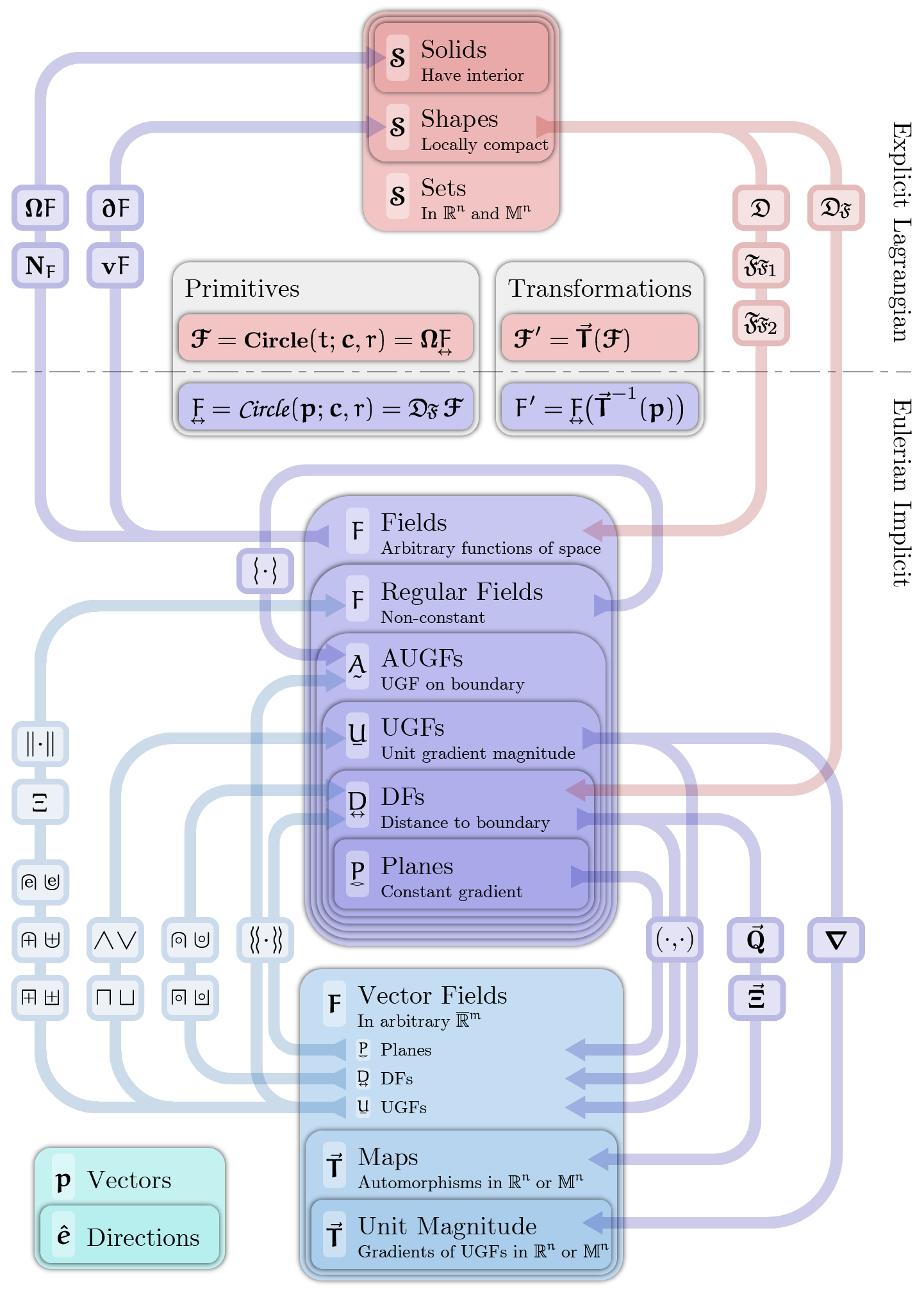
Connecting the Dots
While I’m a fan of John Nash’s work, this portrayal never landed for me. That said, I did question my sanity while working on the diagram below.
Given a few different grades of fields and a set of operators, one might wonder if there’s any structure worth noting. For example, the distance-preserving Boolean maps DFs to DFs, while the minmax boolean map DFs to UGFs. Here’s my attempt to document the structure of the system, with a few operations to be defined in later posts:

A Summary so Far
DFs and UGFs to a shape can only differ in shapes’ normal cones that arise on non-smooth boundaries. In this post and the last, we focused on these sharp (edge-like) regions and offsets to help clarify that all fields with unit gradient magnitude are not DFs. There’s more fun to be had with edges and edge treatments, but perhaps in the next posts we’ll visit some of the tricks that work only with UGFs and some techniques for creating UGFs to new shapes.
Please keep the feedback coming!