For those of us who work in engineering and geometric modeling, “offset” is an everyday operation. We use it in 2D and 3D to produce curves and surfaces at constant distance from other curves and surfaces. With experience, we learn that offset can be failure-prone, especially with precise B-rep solids and meshes. Implicit modeling, in particular, the signed distance field (SDF) representation of shapes, offers robust offsetting, but again, with experience, we learn that the results aren’t always what we expect.
Take these three examples of an offset rectangle, created using three different “line joining” approaches that date back to the early days of 2D graphics and are built into your browser:
The red rectangle on the left uses extensions of the rectangle’s edges. This approach is similar to what we expect from B-rep and most mesh modelers, where extra faces are only added when needed. One might not notice that the offset vertices are actually a factor of \(\sqrt{2}\) farther from the vertex than the sides. In engineering applications, we often prefer the topological simplicity of such naturally extended intersections to geometric correctness.
In the middle, the green rectangle offsets geometrically, with a rounded corner the exact Euclidean distance to the vertex. When modeling with SDFs, we expect these geometric offsets, but the result may surprise engineers who prefer the simplicity of naturally extended corners.
As a third example, although not normally considered a common option during offset in engineering applications, offset can produce a chamfered result. Are there other possibly legitimate options for how one might want to treat a corner?
Offsets and SDFs
When modeling with fields, we often “offset” a field \(F\) as an alternative to offsetting the boundary of the shape \(\shape{F}\) it represents.
(In our notation, one can convert a shape to a distance field via \(\df{F} = \DF \shape{F}\) or extract a shape from the non-positive region of a field via \(\shape{F} = \Shape F\). We also annotate planes \(\plane{P}\), distance fields \(\df{D}\), and unit gradient fields \(\ugf{G}\) to distinguish them from general fields \(F\). The next post will cover these topics.)
We define the offset of the field \(F\) by constant distance \(\lambda\):
\[\func{Offset}_{\lambda}(F) \equiv F - \lambda \;,\]so the distance the zero isosurface moves depends on the gradient of \(F\). One can think of the offset behavior as baked into the field’s geometry itself, not something one can do to the geometry, as with boundary modeling. If we’d like different edge treatments on different edges, somehow we need to produce a fields with the proper behavior encoded in them ahead of time.
For example:
 |
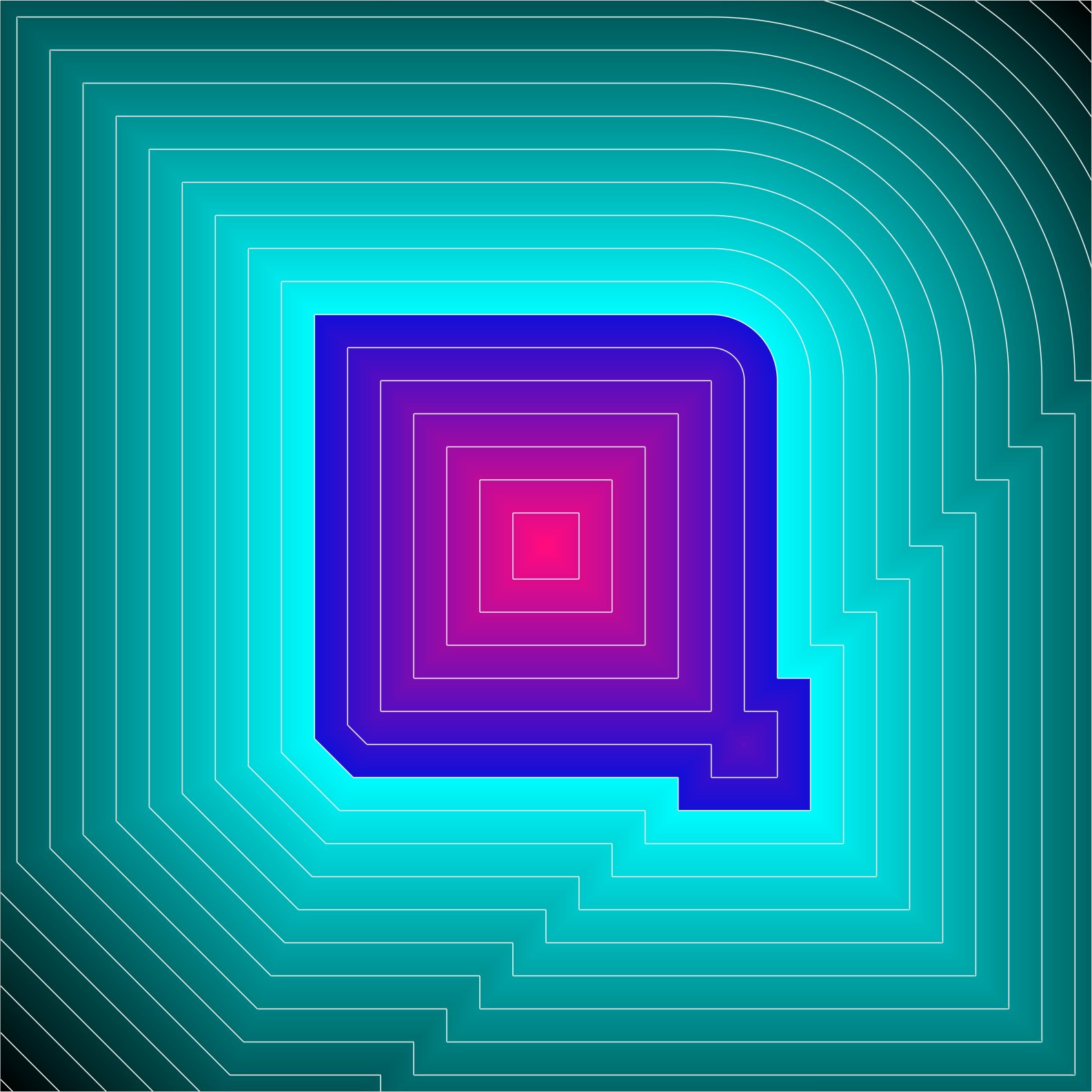 |
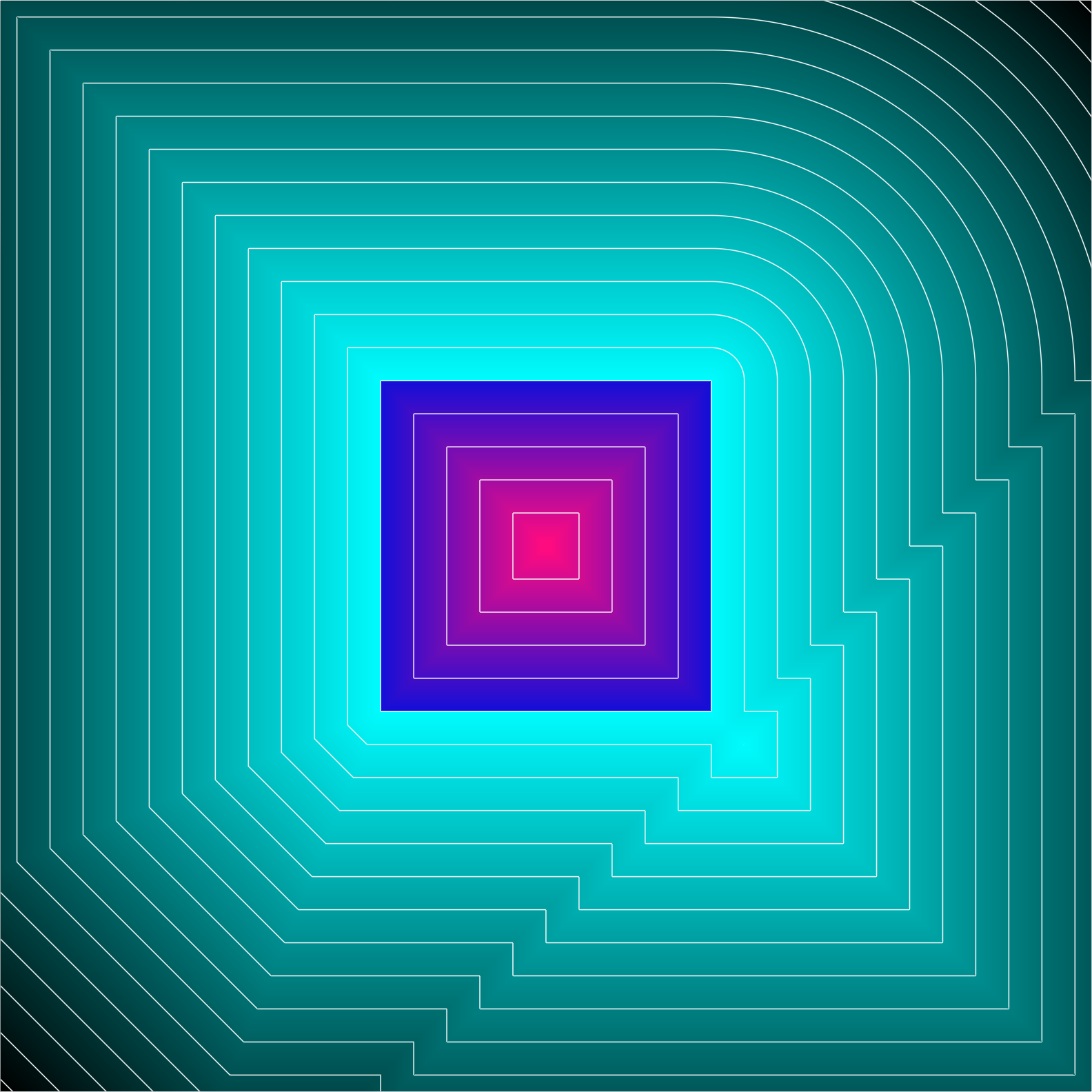
Clearly, only the top right corner represents an SDF. In this example, the gradient, where defined, always has unit magnitude, as observed by the 1:1 slope in the field’s epigraph, \(\planeSm{z} - F(\planeSm{x}, \planeSm{y})\):
A similar situation presents itself in 3D. How the edges of the cube propagate when this spherecube is rounded is predetermined by the field surrounding the cube, yet it’s not visible on the nominal geometry:
 |
 |
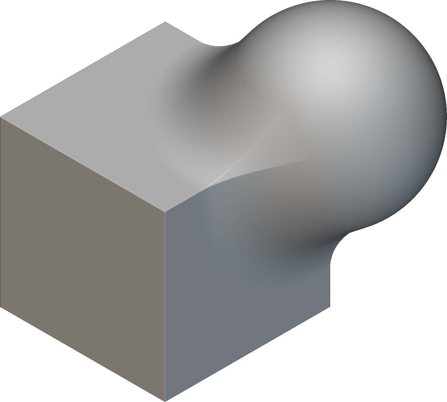 |
The left option is most common with B-rep modelers when rounding an edge, and some provide the option to round the blend, as seen in the center. UGF modeling, however, provides a unique ability to add more control, as expressed with the chamfered alternative on the right.
Introducing Unit Gradient Fields (UGFs)
UGFs, fields with unit gradient magnitude (where the gradient is defined), offer a generalization over SDFs with the appropriate amount of flexibility for many engineering applications. They also overcome the greatest weakness of SDFs: closure.
The offset of a distance field is not, in general, a distance field. Starting with a SDF, if one offsets a convex edge inward or a concave edge outward, the result is a field that no longer represents the distance to the isosurface. (We’ll dedicate a post on this topic soon, but if you wanted an exercise, this would be it.) Similarly, as observed by Inigo Quilez, Booleans, as produced by \(\min\) and \(\max\), do not produce distances. Most other common operations, including blending, smoothing, interpolating, variable offsetting, warping, and even scaling all can introduce artifacts that cause subsequent operations to behave unpredictably. Finally, we can also construct UGFs from other UGFs in ways that are not possible with SDFs.
Over the past year or so, I’ve been gathering my implicit modeling practices into a manuscript unified by organizing principle of UGFs and how they relate to SDFs and their relatives. Now that the book has achieved critical mass, I thought I’d start to introduce UGFs thought a blog series. With the release of nTop 4.0 and its new spherecube and UGF themed logo, as well as in anticipation of conversations at CDFAM 23*, it’s time to start talking about the project!
 |
 |
* Note: while the nTop logo, as most of the images on this page, was designed in nTop, the CDFAM logo appears to have been generated using machine learning.
Example of the power of UGFs
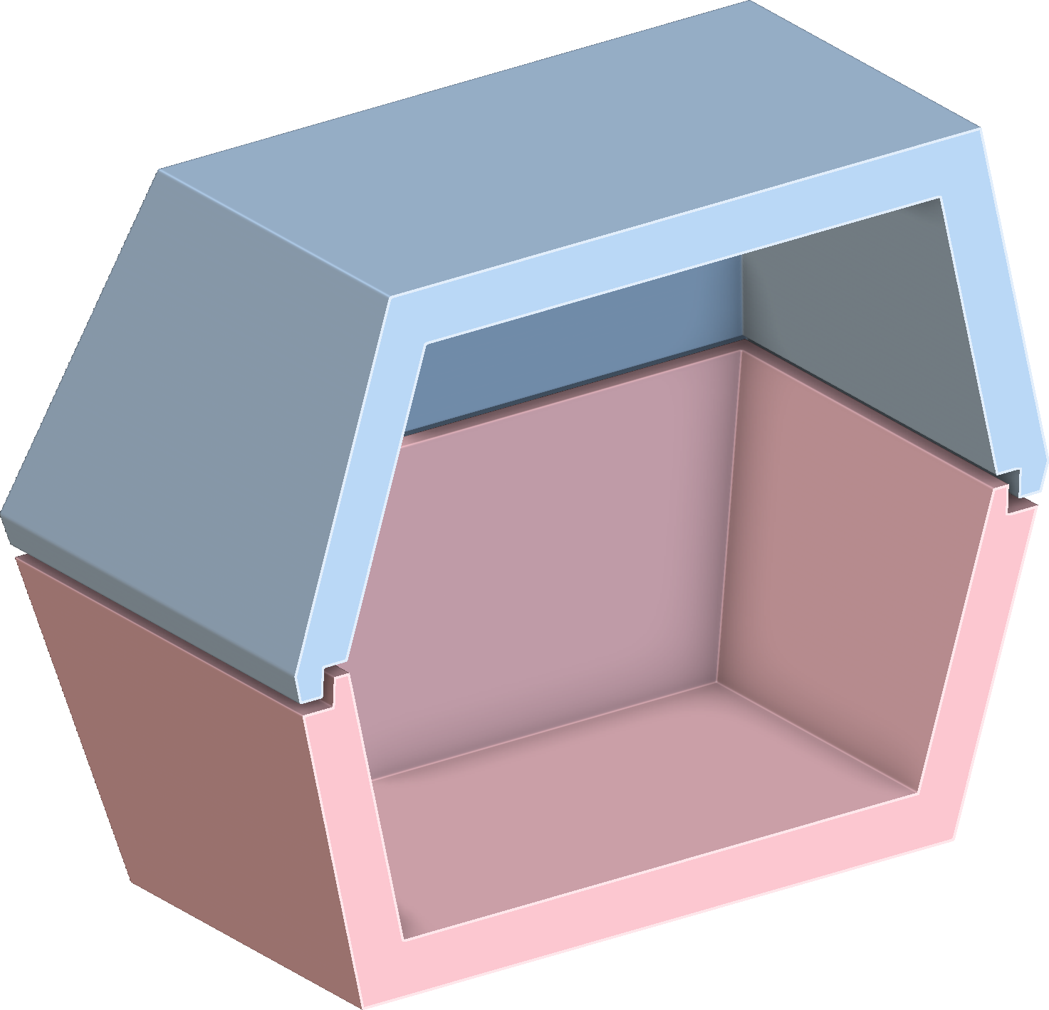
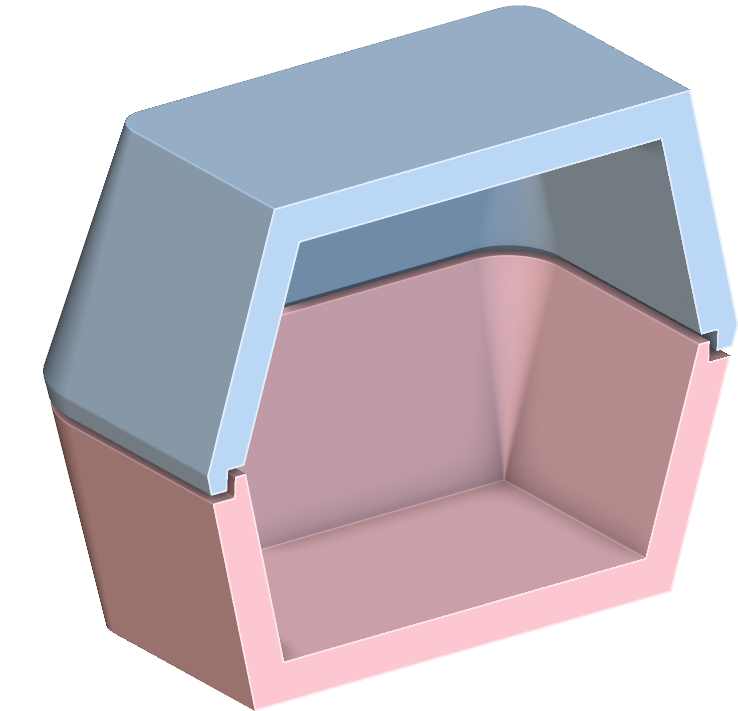
Let’s take a look at a less theoretical example, where we want to control different edges with different edge treatments. Here, we’re also using UGFs to produce drafted faces and a lip feature, as common in molding applications.
 |
 |
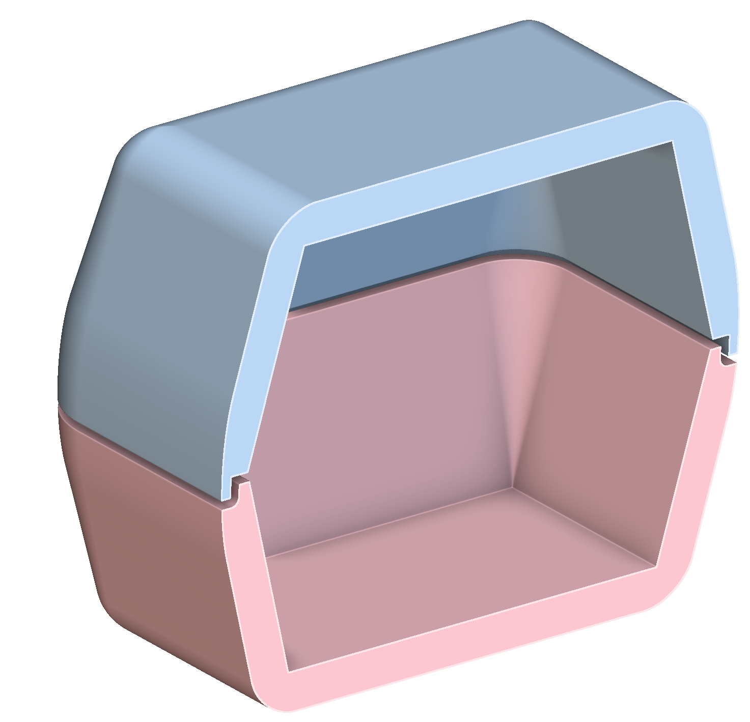 |
Each Boolean operation offers an opportunity to choose what kind of edge treatment is appropriate, establishing downstream design intent. When modeling with UGFs, it is natural to encode such design intent sooner than with explicit modeling, enabling downstream operations to behave predictably and be automated.
What makes UGFs special? Couldn’t we always do these tricks? Yes, but without a resolute focus on maintaining unit gradient magnitude, the results would not produce the constant offsets, circular rounds, and predictable results we associate with engineering software.
UGF Blog series
So stay tuned through June as I walk you through more explanation of the above and through diverse application such as:
- How to use UGFs to condition fields for downstream use when producing lattices, edge treatments, and thin-walled geometry.
- Parameterizations possible from UGFs, such as the two-body field and the orthogonal sum and difference fields.
- Everything you want to know about implicit edge treatments, including rolling-ball blend and chamfer.
- Distance-preserving ramp and other transformations.
- Curve-driven and isocline draft.
And any discussion topics that I hope come up in conversations along the way!
Summary
So to summarize: UGFs are like SDFs but are more useful, enabling a more expressive language for implicit modeling in engineering and closure in modeling with distance fields. By focusing on UGFs instead of SDFs, we can put implicits to work in more engineering applications.
Closing image: multiscale, spatially-varying FDM/FFF infill with constant weld offsets:
