This post originated from conversations with Luke Church, GCL and Brad Rothenberg, nTop. It now includes significant contributions and feedback from: Mark Burhop, Sciath aiM (from whom we anticipate a nuanced paper on this topic); Jacomo Corbo, PhysicsX; Kiegan Lenihan, xNilio; Peter Harman, Infinitive; Saigopal Nelaturi, C-Infinity; Hugo Nordell, Encube; Alex Huckstepp, Uptool; Neel Goldy Kumar, Intact Solutions; Blake Reeves, Pasteur Labs; Andy Fine, Fine Physics; Kyle Bernhardt, Collectiv; and Claude 3.5 Sonnet.
Executive Summary
The future of AI in engineering won’t arrive as a single superintelligent design system. Instead, 2025 will see the rise of specialized AI agents that work alongside engineers throughout the product lifecycle — simulating assemblies, automating documentation, optimizing components, and configuring supply chains. These agents, operating both within existing tools and through new platforms, represent a fundamental shift in how we develop products, one that promises to dramatically accelerate and enhance the engineering process. Success will require solving key technical challenges around security and agent coordination. GCL is convening industry leaders this spring to tackle these challenges together.
Vision
The engineering industry’s vision for AI-powered design tools seems to mirror science fiction, from Star Trek’s Holodeck to Tony Stark’s workshop. The narrative follows three steps:
- An engineer declares intent, describing a design objective, its constraints, and performance goals;
- The computer synthesizes a complete design proposal, from geometry to materials to manufacturing; and
- Through rapid iteration and feedback, the engineer and AI converge on an optimal solution.

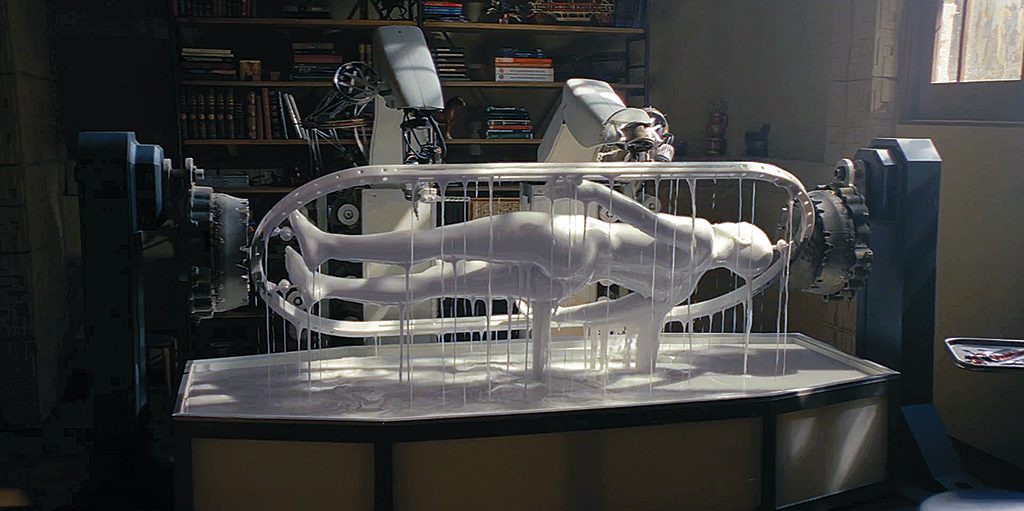
The crew of the Enterprise collaborates with The Computer to reconstruct a medical table in the Holodeck. Although this episode of TNG jumped the shark, this scene influenced me greatly.
This vision parallels what we’re seeing with AI art tools like MidJourney and Stable Diffusion: creative systems driven by geometric suggestions, natural language prompts, and iterative refinement. Could engineering tools evolve similarly, adding physics, manufacturing constraints, and performance optimization to the mix?
The path to this future builds on three generations of generative engineering software:
-
Procedural Generation: While early automation such as AutoLISP and Pro/Engineer elevated geometry languages from low-level modeling instructions to occasionally capturing true design intent, such business logic requires extensive programming or additional product layers like expert systems or configurators.
-
Topology Optimization: These tools synthesize geometry directly from engineering requirements and boundary conditions. While powerful for specific use cases like lightweighting parts, current systems require significant human effort to produce manufacture-ready designs.
-
Machine Learning: Emerging ML approaches have shown promise in architectural applications like space planning and restoration. However, they’ve yet to achieve comparable success in mechanical engineering, where physical constraints and manufacturing requirements pose greater challenges.
Each of these approaches will evolve into more sophisticated agents that proactively participate in the design process as well as interfaces supporting such agents. But to understand how this transformation will actually unfold, we need to look beyond the Hollywood vision to the day-to-day realities of engineering work.
Reality
I entered this industry inspired by the sci-fi generative vision, but quickly discovered a different reality: engineering isn’t primarily about raw ideation. The mechanical industry is dominated by reuse, the architecture and construction industries by codes, standards, and communities of practice. Synthesis seems seductive, but must conform to existing designs and established practices. Although the engineering industry has achieved significant standardization, for standards bodies and regulatory frameworks, AI may run afoul of copyright and licensing constraints.
The data challenge runs deeper than just access. High-quality engineering data remains locked in proprietary PLM and BIM systems, and even when available, frequently fails to capture actual design intent. While the abundant public images that feed MidJourney and Stable Diffusion are relatively self-contained, engineering datasets remain siloed in a babel of proprietary, binary file streams. More fundamentally, while evaluating an AI-generated image is nearly instantaneous, validating an engineering design can be more expensive than creating it “correct by construction” in the first place. This explains why engineering embraces standards not just from tradition, but as a practical necessity for managing complexity and cost.
Yet at GCL, we’re seeing an encouraging trend: a constellation of startups are finding ways to extract value from this real-world data, becoming useful collaborators in the product development process. While these AI tools currently run independently from engineering databases, 2025 will mark a turning point as they begin operating autonomously within CAD and PLM systems.
The major wave of AI in engineering won’t come from a single massive system that realizes the sci-fi vision. Instead, it will emerge through many specialized agents, each adding value to, and perhaps transforming, existing systems and workflows.
Applications
If engineering’s AI future lies in specialized agents rather than monolithic systems, how will this transformation unfold? Let’s examine the emerging applications in order of technology readiness, starting with one of the oldest tools in engineering: surrogate modeling.
Surrogate modeling
At its core, surrogate modeling resembles sophisticated curve fitting: something as common as interpolating thermodynamics tables or a floating point trig computation. But modern surrogate models do more than just fit complex mathematical functions to high-dimensional data. In fields like astrophysics, surrogate models aim to reproduce the underlying physical processes themselves, not just their outputs. This contrasts with most AI training, which typically focuses on replicating outcomes without modeling the generative process. When today’s AI experts talk about “training a model,” they’re often building outcome-focused approximations at unprecedented scale.
Surrogate modeling supplants slow or iterative processes with instantaneous answers. Companies like PhysicsX, Pasteur Labs, and Neural Concept are applying this approach to accelerate physics simulations and predict experimental outcomes, while multi-disciplinary optimization tools like Noesis Optimus, Siemens PLM HEEDS, ANSYS ModelCenter, and Esteco ModeFrontier integrate surrogate models into broader system optimization workflows. As the surrogate models become increasingly comprehensive, complex workflows can be led with models.
For example, the aircraft design process I learned in school starts with payload, speed, and range requirements that drive initial wing sizing calculations. Airfoil choice leads to drag and reaction forces, which inform iterative cycles of aerodynamic and structural analysis, progressively refining the design while balancing performance metrics against practical constraints until reaching an optimal solution. We were taught techniques for shortening the inevitable iteration loops.
PhysicsX’s ai.rplane demonstrator obviates such iteration. The model subjects a set of plane-like geometries to virtual wind tunnel tests and captures performance as well as sizing metrics, plotting the results on some flattened latent space. Perhaps, in the near future of systems engineering, identifying iteration loops becomes a kaizen event for surrogates?
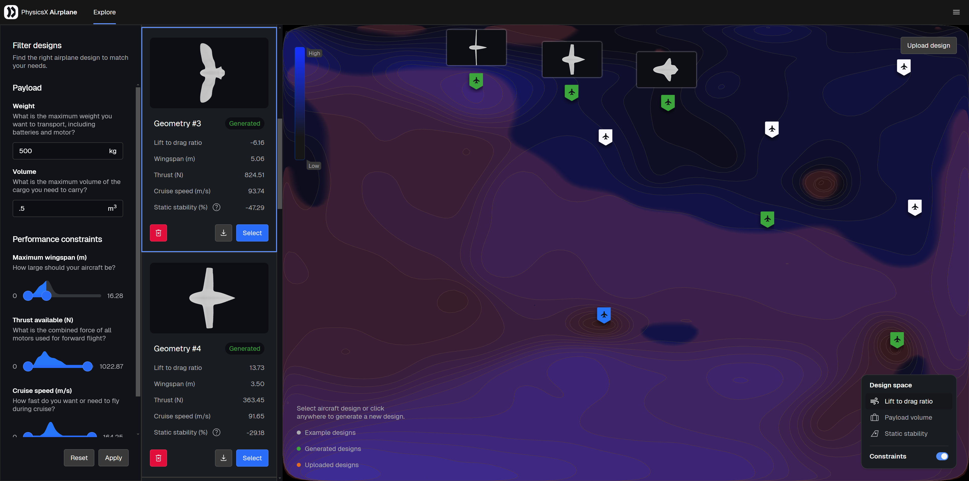
In this screenshot from ai.rplane, I’ve sampled some points in what appears to be a 3D projection of latent aircraft space, with a bird of prey selected. The red region shows airframes too small for my payload’s volume. I overlaid three thumbnails above the samples at the top to show how the latent space appears to interpolate the shape space, with the slenderest too cramped for the desired payload.
The evolution to agents takes this further: surrogate models become active participants in the engineering process. While these predictions still require validation for critical decisions, they enable continuous exploration of complex design spaces that would be impractical to simulate directly. The same approach applies to supply chain optimization, where surrogates can model the interactions between cost, availability, and performance across thousands of components.
Quoting, costing, and time estimation
Over the past dozen years, I’ve had a close look at about a dozen cost and time estimators for CAM, 3D printing, and production processes. Manufacturing marketplaces like Xometry, Protolabs, Meviy, and Fictiv compete on some Pareto curve of price, turnaround, and time-to-quote; they all have accumulated valuable training data from millions of parts.
Neural-net based estimators aren’t new: they’ve shipped on manufacturing hardware for at least two decades, with 3D printer vendors using them to predict print times and material consumption. MES systems have extended this approach to more complex manufacturing operations, learning from actual production data. Keep an eye on startups like Encube and Uptool to deepen AI and ML’s role in manufacturing unit economics and arbitrage.
AI agents can “left-shift” cost estimation: moving it earlier in the design process, directly into CAD and PLM systems. Users could receive continuous cost updates as they design, similar to how simulation feedback appears at the end of their feature tree. While some CAD add-ins already provide real-time quoting, these capabilities remain rare differentiators. Standardized protocols for cost estimation agents would make such services ubiquitous, benefiting both customers and vendors.
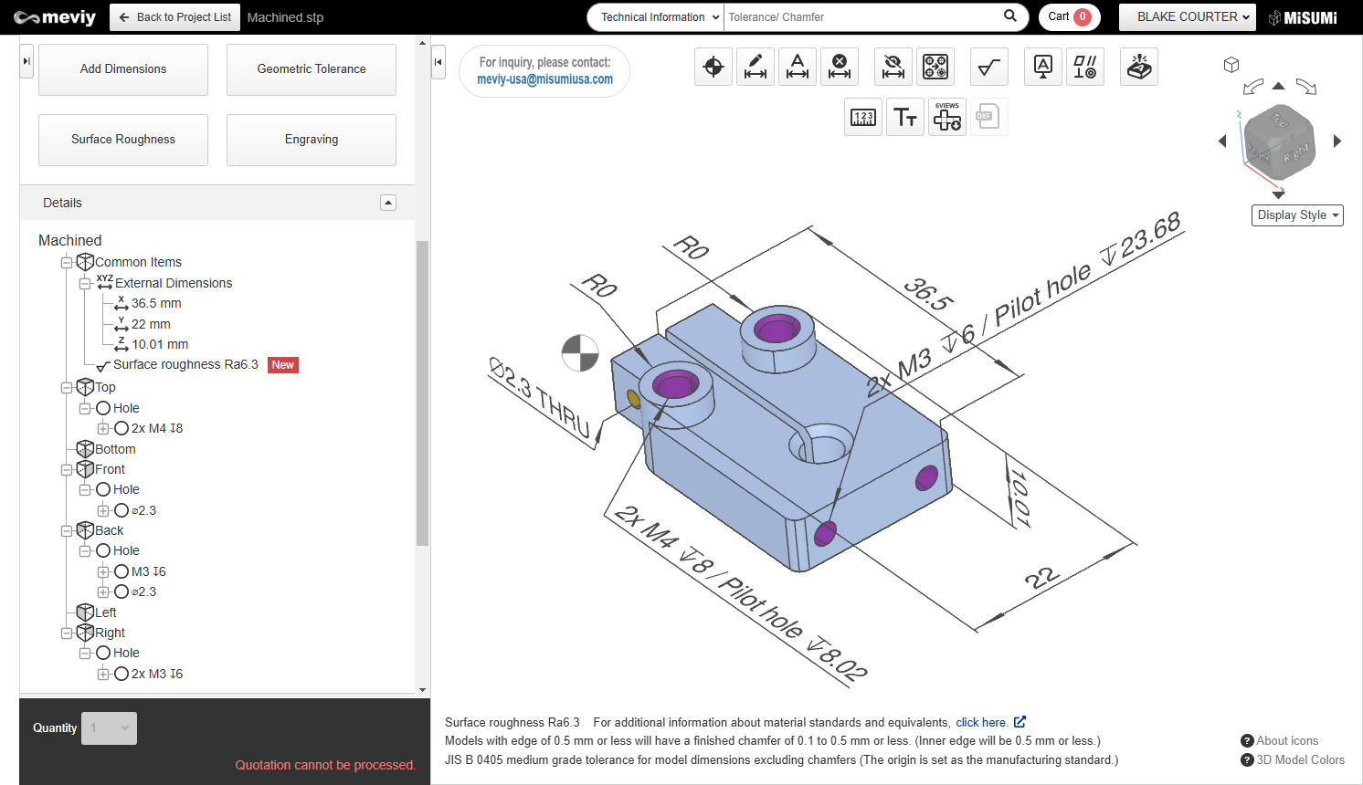
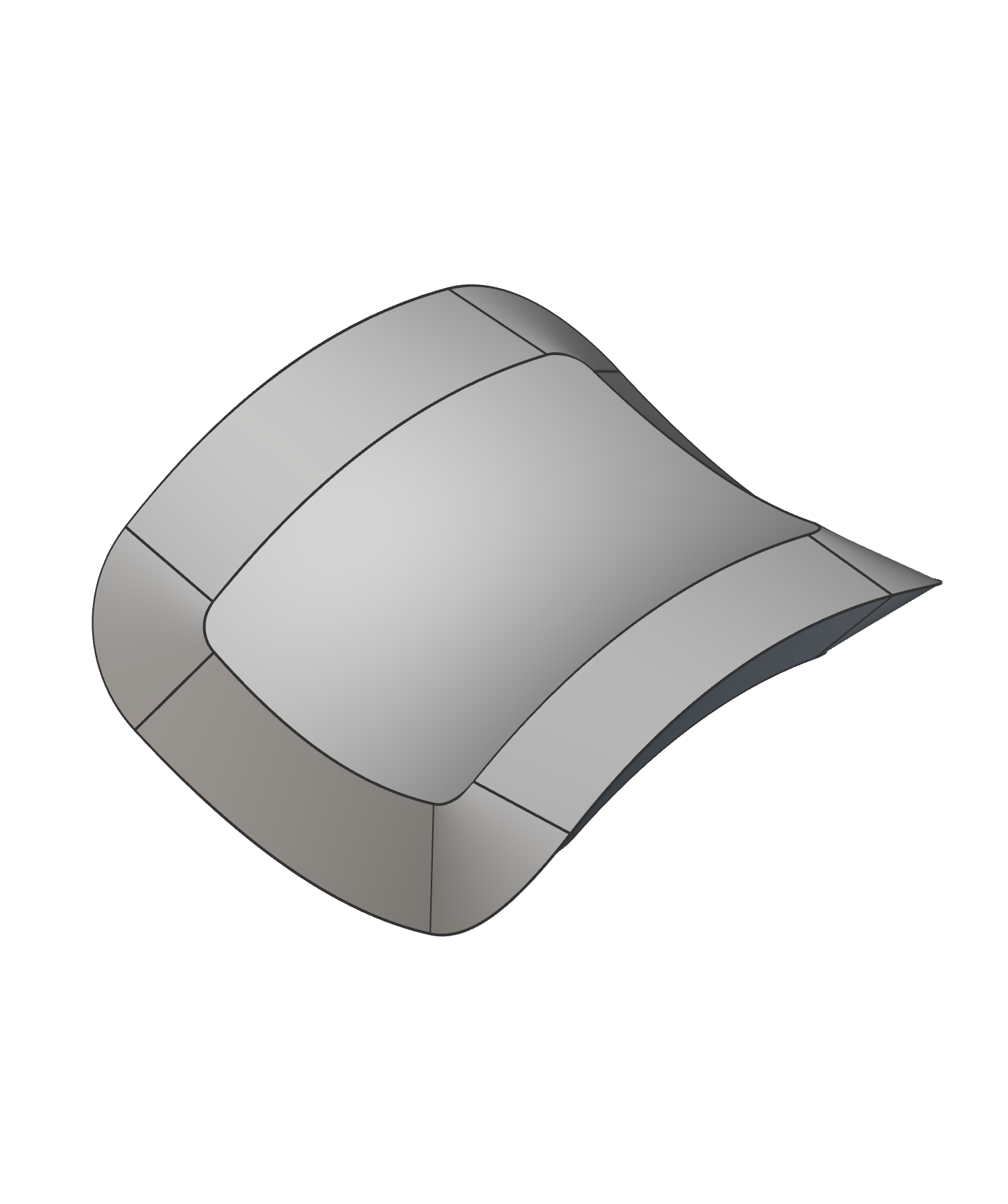
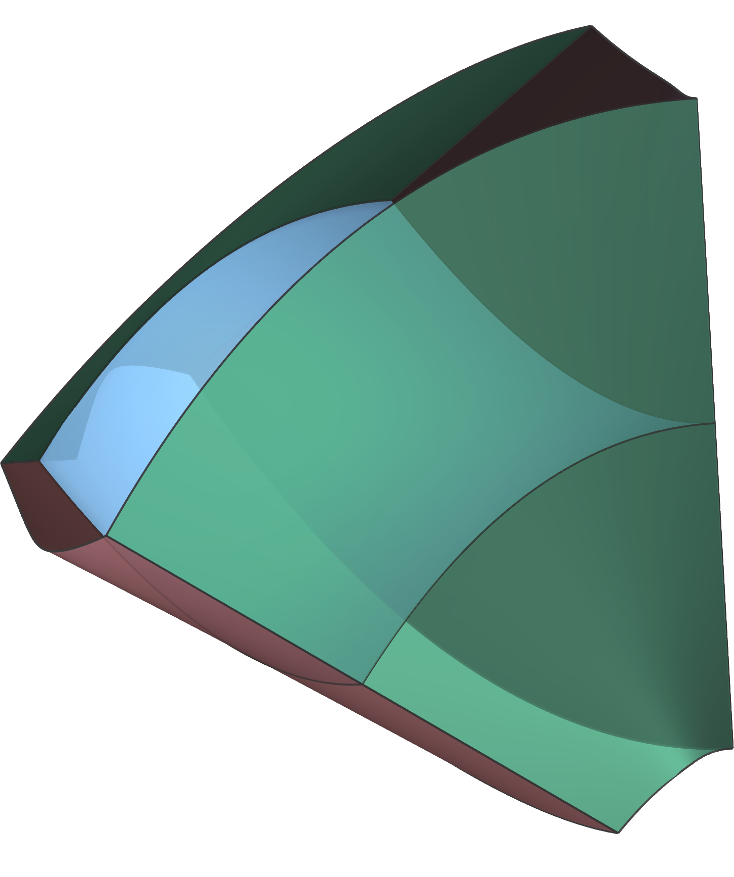
Misumi Meviy’s CNC quoting tool automatically recognizes manufacturing features and shows you the manufacturing plan. I expect they will be able to handle this slitting feature someday, as well as the hole before it.
What about more specialized machine shops? Uptool is building automation to interpret quotes, including nuances like tight tolerances that are not handled by the commodity vendors, all while keeping experts in the loop.
A reasonable machinist might also recommend a design change. The manufacturing industry has long lamented designers’ apathy of design-for-manufacturing. Like a good machinist, Encube suggests small design changes that lower manufacturing costs. Could an approach like Encube’s finally left-shift DFM into CAD?
Drafting
Sometimes, a CAD part isn’t enough to produce a quote, but a drawing usually is. I’ve recently been helping engineer a family of fancy brackets for some friends’ design project that called for interlocking tapered pockets, a geometry case that broke the quoting tools I mentioned above. The local CNC shop was happy to take the work, but needed drawings. I tried to get away with only detailing the most complicated one, and hoped they could take it from there. But no, they needed a drawing for every one. Then, after sending all the drawings, they asked me for tolerances, which meant I had to mostly redo the first, most complicated drawing because most of my dimensions had disappeared. Deducing the tolerances became a gut-wrenching process not so much for the math anxiety, but because I feared their sarcasm for a tenth of a thou on those tapers! Somebody “intelligent” probably saw that coming, and sent me a follow up not to bother with the tolerances after all.
This story illustrates three universal truths about engineering drawings: everybody wants them to be complete, accurate, and up-to-date; nobody wants to make them; and they often contain low-confidence information dressed up as precise specifications.
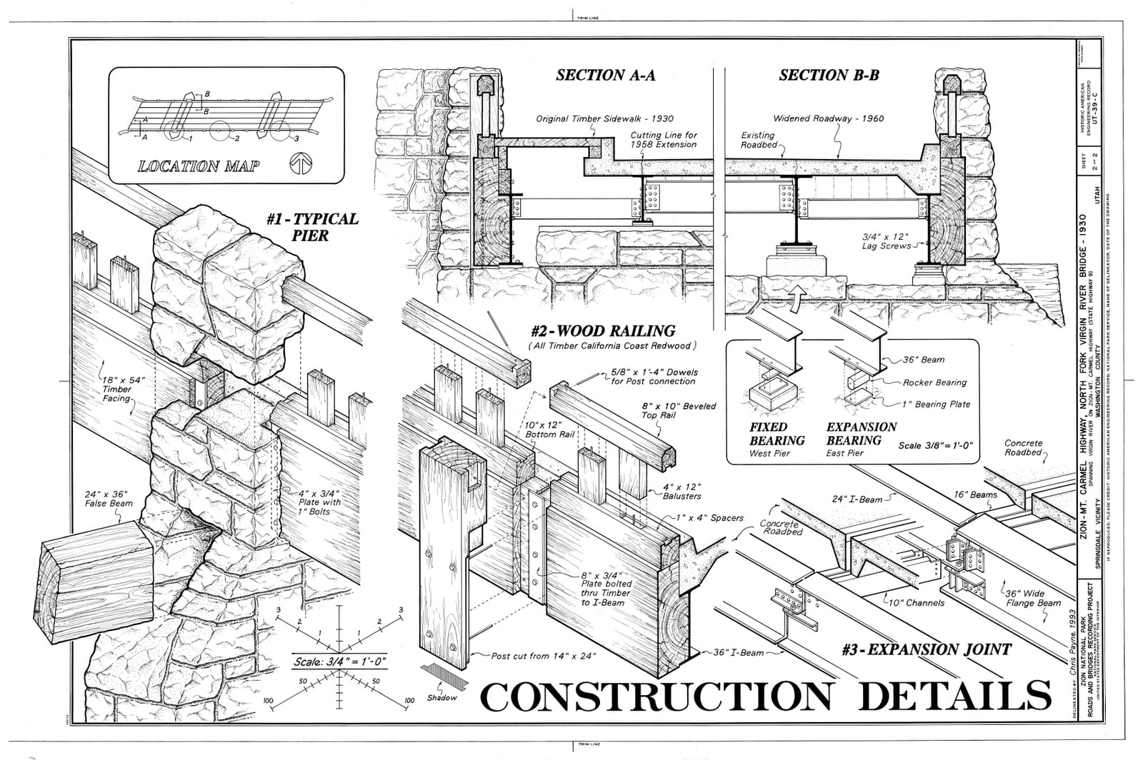
Apparently, a human-drawn drawing, via Spencer Wright’s et al’s excellent newsletter, Scope of Work. IMO, it could use some whitespace.
Enter generative AI drawings. Companies like Hanomi, Drafter, and Swapp are showing impressive results that go beyond automated dimensioning; they’re building foundation models for geometric dimensioning and tolerancing (GD&T), by necessity solving sophisticated generative problems to deliver drawing synthesis. These systems will likely expand to generate geometry, especially basic parts like plates, brackets, and other common components.
Packaged as agents, these capabilities will integrate directly into our CAD workflows: finished drawings appear automatically at the bottom of our feature trees, complete with appropriate GD&T back-propagated to the 3D model. The agents could even suggest part variants optimized for different manufacturing processes, each with associated quotes and lead times.
Mark Burhop anticipates that similar downstream agents will left-shift much more, expanding from manufacturing agents that create interchangeable parts across manufacturing processes or vendors to predictive serviceability, repair, and wear, and sustainability and circularity.
Supplier agents
In PLM and BIM, most designs are assembled from standard components, such as linear rails, aluminum extrusions, and motors in machine design, and studs, windows, and curtain wall systems in AEC. For commodity items like fasteners and materials, CAD systems may provide integrated databases of “smart” components, suggesting possible interaction paradigms. However, this approach misses nuance in more competitive technical components, which is why suppliers often attribute their success to high-acumen sales engineers.
Some of the highest-growth engineering software startups, like Vention and Higharc, recognize this reality: they’ve built custom CAD systems where the software becomes part of the overall product experience. Instead of requiring their suppliers to purchase and learn software up-front, the future end-users of the actual machines or homeowners can immediately start configuring solutions.
For mainstream engineers, designing a machine or building remains an odyssey through drawings, CAD files, and sales literature. LLMs and generative 3D technology promise to transform this experience by transforming disparate product data into agentic actors in CAD, PLM, and BIM systems.
Consider designing a custom manufacturing device that needs an XY table, common in 3D printers and CNC machines. You want to optimize between rigidity and speed across different rail configurations and drive systems. Companies like Misumi offer sophisticated configurators, but you still need to make detailed decisions about pre-loading and seal wear just to get a STEP file that requires manual assembly. And that’s just the first rail.
Imagine instead: you draw a box in your CAD assembly, specify your end effector load, and let supplier agents compete for your business. You might see variations from Misumi, THK, and HIWIN, along with unexpected proposals from vendors you hadn’t considered. LLMs handle your questions like experienced sales engineers, reconfiguring designs on-the-fly, complete with lead times and volume pricing.
These systems, funded by suppliers’ sales and marketing teams, raise interesting security questions: How do we enable agents to make decisions based on CAD data without risking intellectual property? Could suppliers optimize production by analyzing where their components appear in designs? Will trusted third parties be needed?
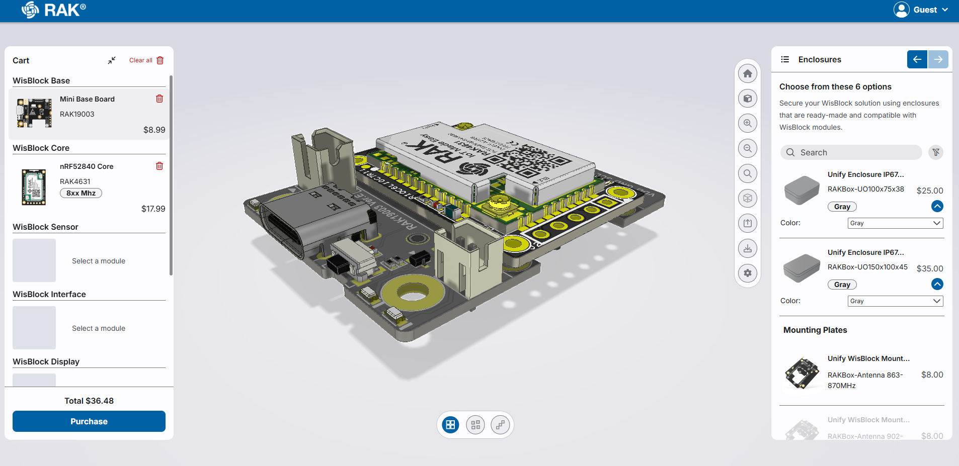
Meshtastic Designer, an IoT design tool powered by Infinitive, a configurator platform that generates designs from engineering requirements while also informing e-commerce and ERP.
Infinitive appears to be pioneering this approach in discrete manufacturing, while several startups explore AI-powered AEC marketplaces. This model of embedding design software into revenue streams is gaining traction among engineering software startups. If you have a high value service that could be delivered as an AI sales agent, please let us know.
Simulation
When SpaceClaim started to take off with simulation users, I had the opportunity to problem-solve with all sorts of engineers on a daily basis. Given that all models are wrong, I’d ask questions like “how do you know that your results are accurate” and “how do you build confidence that you’ve handled all the cases,” to which I’d hear answers like “my results aren’t accurate, but my derivatives have the right sign” and “there’s no way we have enough time to handle all the cases we can think of.” And some everyday engineering validation requirements like drop testing and assembly-level resonance testing seem like simulation fantasy.
We already discussed surrogate models, which can build confidence when connecting simulation results to empirical data. Using various forms of neural networks and similar approaches, companies like PhysicsX, Pasteur Labs, and Neural Concept may accelerate results by two to six orders of magnitude. These vendors are developing and releasing increasingly advanced and differentiated models, much like how OpenAI and Claude.ai are competing on LLMs.
The next step is embedding this capability directly in the design process. Prominently in AEC, Autodesk has implemented surrogate models to deliver near-real time CFD visualization in their Forma product. Simulation agents will continuously analyze CAD assemblies, working from the PLM context to evaluate everything in sight. Interfaces and kinematics will emerge automatically from geometric placement; quick modal studies will detect gaps and interferences like a real-time spell-checker. Combined with increased cloud and GPU resources, we can finally start to cover all the simulation edge cases. Perhaps we can even measure the completeness of our simulated test coverage similarly to how the software industry measures code coverage in QA.
These agents will provide feedback similar to how modern programming environments guide developers: immediate, context-aware, and actionable. xNilio (stealth; material used with permission) demonstrates this with their product-level agent system, while companies like Intact Solutions and CoreForm show how meshless simulation can directly use adjacent parts in assemblies as boundary conditions. The SimSolid technology at Altair already excels at these assembly-level problems.
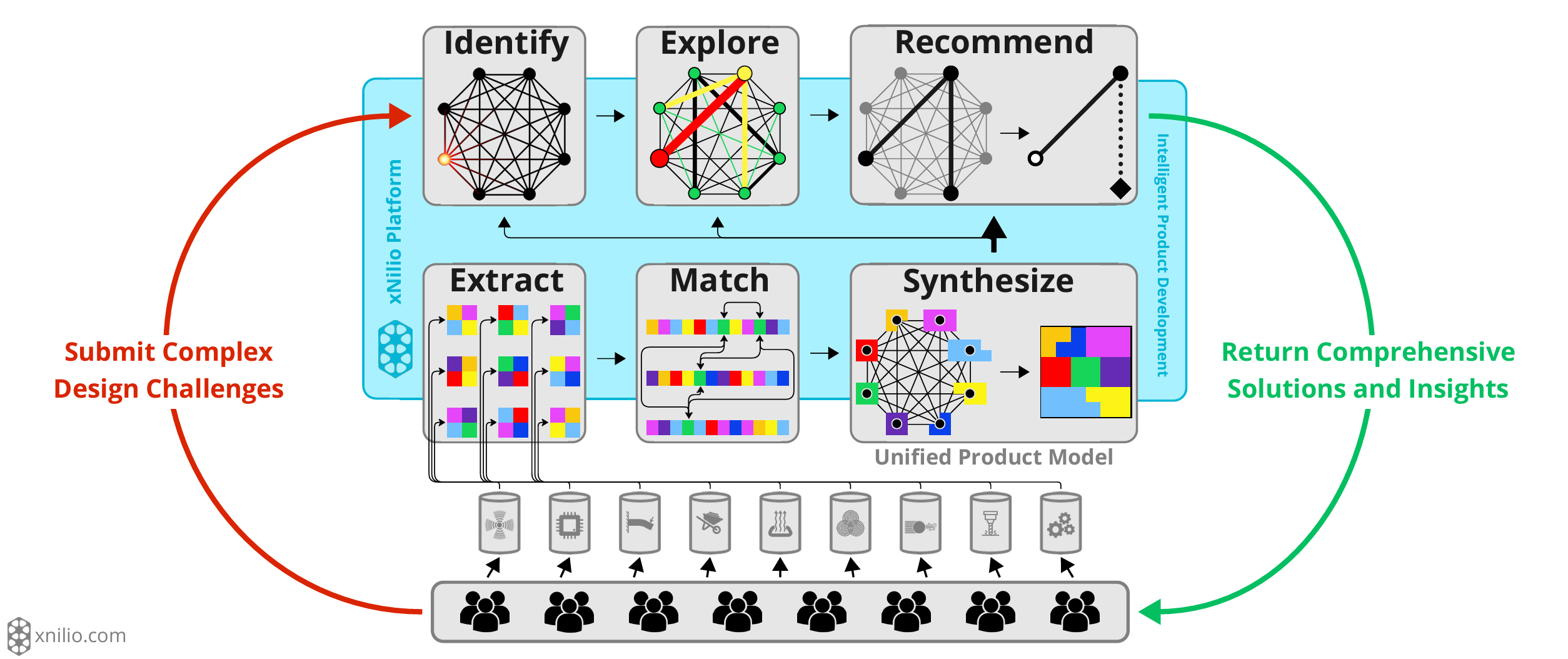 xNilio identifies patterns and simulates product-level problems, functioning as a continuous, offline design review.
Large OEMs often process enormous volumes of product revisions per year, creating an overwhelming flow of changes that must be verified for each product and configuration. Each change has the potential to disrupt assembly instructions, impact fitment, or require revalidation for multiple product options. Engineers face the difficult task of testing every configuration, which is extremely slow without automation. C-infinity and Dirac are producing approaches to navigate and validate the configuration space of complex product assembly.
The challenge isn’t just technical but interactional: how do we present all this intelligence without overwhelming engineers? Simple notifications, as I learned from the early overuse of Slack integrations, can quickly become noise rather than signal. Similarly, in software development environments, it took about two decades for static analysis to evolve into useful autocomplete. The future might lie in more subtle interfaces: annotations in digital mockups, contextual reports, or selective alerts based on risk levels. But we’ll need to carefully balance comprehensive analysis against the practical limits of human attention.
Is generative CAD ready for agents?
But when will CAD systems draw, or at least autocomplete, our parts for us? We’ve seen success in architectural applications like automated office layout, and topology optimization has given us countless lightweight brackets. These victories hint at broader possibilities, but the path to true AI-driven design may run through some familiar territory.
Parametric generative
Before PLM, we called the mechanical CAD industry “mechanical design automation.” Starting with Pro/Engineer, parametric, history-based CAD tools could produce infinite variations of a design using a parametric recipe. These “parametric generative” systems encompass computational design, expert systems, and anything knowledge-based, procedural, or declarative, including programming languages. Field-driven systems like nTop achieve superior reliability through implicit modeling, while workflow-focused platforms like Synera excel at integrating disparate systems.
Knowledge-based engineering
Outside of mass customization and families of simple components like fasteners and bearings, knowledge-based engineering first appeared in tooling design like molds, dies, jigs, and fixtures. Sophisticated experts needed to program the CAD systems or author reusable “templates,” and such investments make economic sense in high end applications.
In the architectural and design world, the “computational” design paradigm celebrated dataflow models starting with Generative Components, Dynamo, and Grasshopper. Most modern architecture and industrial design with thematic, varying patterns result from artists exploring these tools. The “dataflow” environments navigated by computational designers descended from tools used by electronic musicians, such as Max/MSP, and foster subjective, experimental workflows.

Max/MSP: navigating the void between DJ and computational designer since 1985.
Closed loop optimization
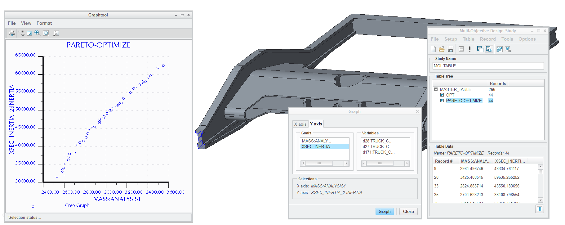
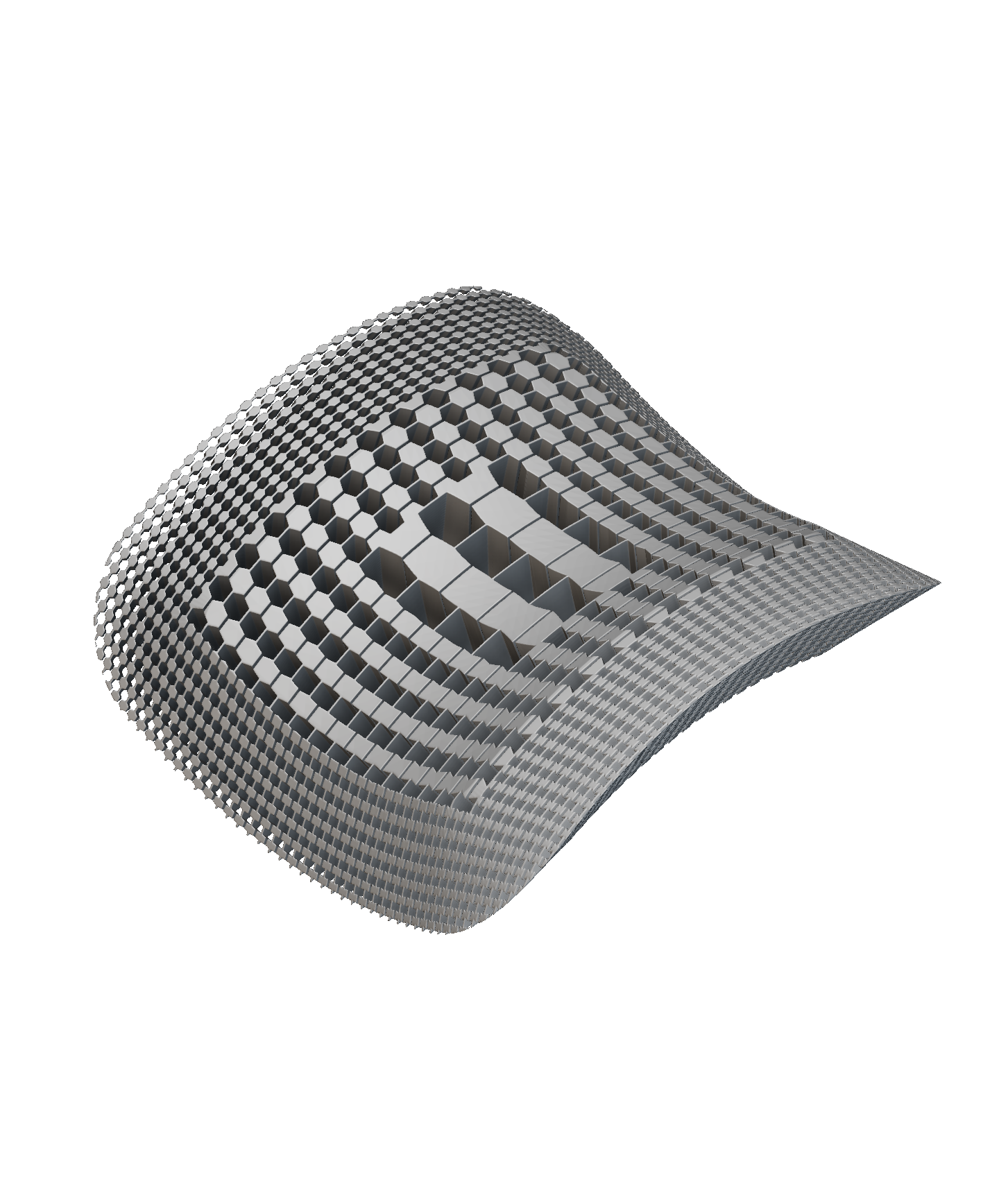
Coupled with simulation, it’s a common practice to run experiments with myriad samples to chart Pareto fronts (optimal sets) for how various parameters affect product fitnesses, or perform a gradient descent to find local optimality, as introduced with PTC’s behavioral modeling. Leap71’s pure code approach exemplifies the power of this methodology.
Topology optimization offers another optimization path using heuristics to produce optimal parts with simple solvers. nTop adds spatially varying control to parametric modeling through their trademark “field-driven design,” broadening the practice to more geometries and fitness functions. Machine learning appears poised to revolutionize these optimization technologies, particularly through neural implicits and a better understanding of design context. For example, TOffeeX is applying this technique to multiphysics systems, in some cases replacing what was done with surrogates just a few years ago, and InfinitForm is improving compatibility with CAD representations.
Geometric optimization continues to expand beyond individual parts to entire processes. Companies like Atomic Industries are taking a vertical approach, building optimization knowledge in layers to complete manufacturing pipelines for optimal control over quality and throughput.

Leap71’s aerospike engine appears to use parametric optimization and inverse engineering as part of its intelligence model.
Diffusion-based industrial design
Recently, the term “generative” has gone mainstream in art and graphics design. Why can’t we just diffuse mechanical designs from prompts and sketches?
The answer lies in engineering’s sensitivity to small changes: slight geometric modifications can dramatically affect performance, especially when they alter topology. While art models can smooth over such discontinuities, engineering cannot. However, industrial design, the most artistic side of engineering, offers promising territory for diffusion models.
Tools like Vizcom already demonstrate the potential of diffusion for industrial design sketching. While 3D applications remain unexplored, the future seems clear: we’ll soon send the internal components of consumer products and simple machines to AI industrial designers who will generate complete enclosures, including attachment points, fasteners, latches, and hinges. Mold shop agents will then generate the necessary tooling. Why not have designer agents in your CAD system, wrapping your chassis with different design suggestions.
If you’re interested in building a generative industrial design startup, let’s talk.
The agentic engineering ecosystem
Is a CAD agent just a CAD add-in on steroids, or are new approaches needed to support agentic product development processes? While agents will certainly need access to CAD and PLM APIs, if we treat them as simple services, like file translators, we may miss their transformative potential. The integration of AI agents into engineering workflows raises fundamental questions about architecture, security, and process.
Data ethics
Consider privileges and autonomy: for example, should an interference-checking agent have the authority to automatically edit parts and schedule design reviews? Could it initiate engineering change orders? Software development already embraces automated quality checks that can reject submissions and automatically recommend some categories of minor changes, suggesting a model where agents operate within supervised workflows. The challenge lies in balancing autonomy with control.
Access and security
Security presents another critical dimension. As agents process proprietary design data to deliver insights, they must do so without exposing intellectual property. AI systems engineering requires careful consideration of security boundaries and data access patterns.
Even if the data is available, is it presented in a useful form? How will we analyze and prepare it for training, such as via tokenization? Companies such as KeyWard help create automated pipelines for moving data into modern data science techniques.
Scalability
The potential for AI agency extends beyond immediate process automation. Just as agents can optimize individual designs, they might learn broader patterns from PLM datasets: predicting delivery times, forecasting costs, and identifying process improvements based on how engineering data evolves over time. “K-ai-zen events?”
These questions highlight a broader transformation in engineering practice. As agents handle routine validation, surface relevant data, and automate tedious tasks, engineers can explore more design alternatives, validate more scenarios, and respond more quickly to manufacturing and supply chain feedback. The result isn’t just improved efficiency, it’s a deeper engagement with the entire value chain from concept to delivery.
Looking ahead, we expect existing CAD add-ins to evolve into agent frameworks, becoming specialized agents with well-defined interactions. This transition will make the tacit knowledge encoded in these tools more accessible to automated systems, creating a richer ecosystem where human expertise can be systematically applied at scale.
Summary
The emergence of AI-powered engineering agents represents a fundamental shift in how we approach product development. Rather than waiting for a single unified AI system to revolutionize engineering, we’re seeing a more organic evolution where specialized agents integrate into existing workflows, each addressing specific aspects of the engineering process, gradually transforming engineering from a purely human endeavor into a collaborative process between engineers and AI systems.
What makes this transition particularly noteworthy is how it preserves and enhances existing engineering workflows rather than replacing them. These agents work within our CAD, PLM, and BIM systems, augmenting rather than disrupting established processes. They’re bringing AI capabilities to engineering in a way that respects the complexity and precision requirements of the field while addressing practical challenges around proprietary data, security, and integration.
As we look toward 2025 and beyond, the key challenge isn’t just developing more sophisticated AI capabilities, it’s creating the infrastructure and protocols that allow these agents to work together effectively. We need frameworks for agent privileges, security boundaries, and supervision that can scale across organizations and industries. The potential impact is significant: faster design cycles, more optimal solutions, reduced errors, and ultimately, better products. But realizing this potential requires careful attention to both the technical and organizational challenges of integrating AI agents into engineering workflows.
Plan for 2025
At GCL, we’re starting to make systems that host agents to analyze and generate PLM data, and we’re aware that many others than those we’ve named are working on AI that could present as or host agents. We’re contemplating a focused, technical workshop in the spring to hammer out solutions to some of the challenges above. If you’d like to participate, please respond here!
]]>


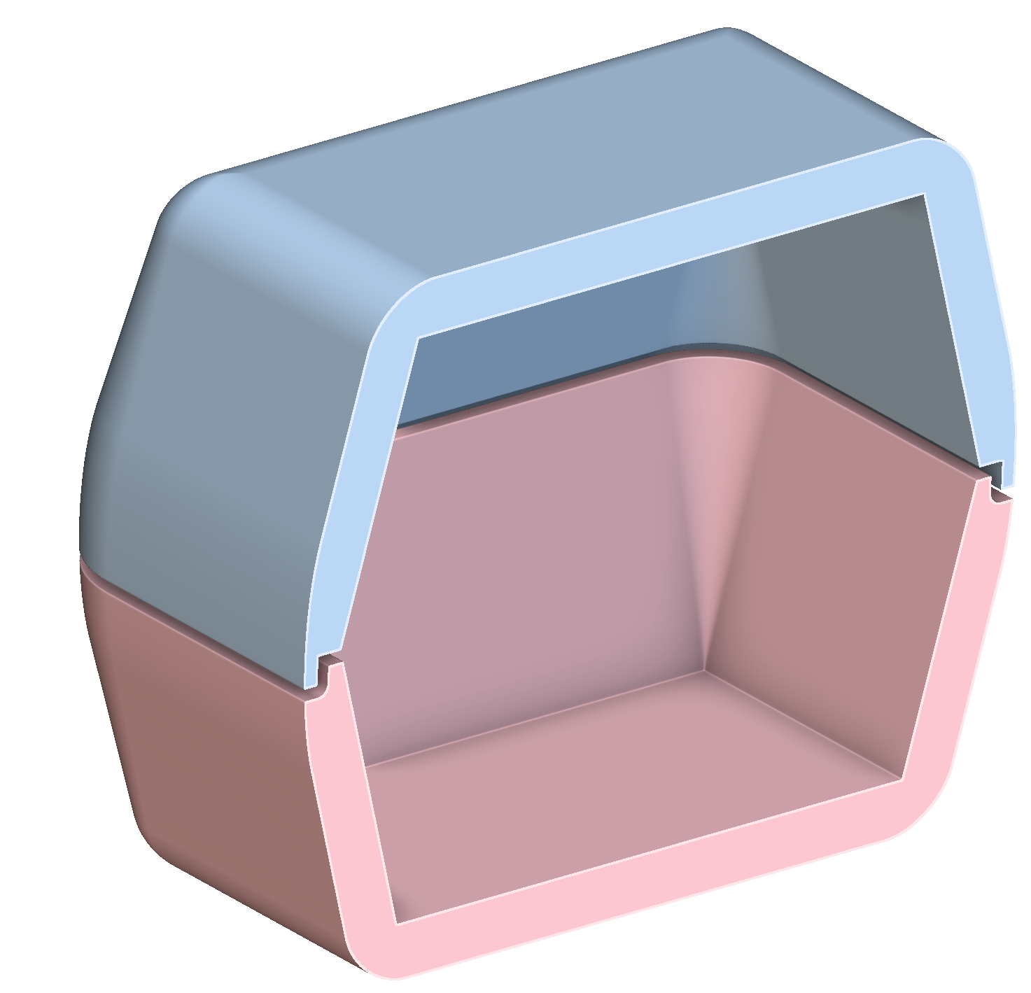
 A swallow with its tail